
This post is part of a series of posts in which I provide the details of each unit I taught post-transitioning to online in Spring 2020 in the Watershed Hydrology class at Kent State University. For more context about the course and my perspective on it, please read the introductory post. [I’ve added some bracketed notes about things I’d change up for a future online offering.]
Learning Objectives:
By the time you’ve worked your way through these materials, I expect you to know how to:
- Explain the relationships between the concepts of gravity drainage, capillary water, adsorbed water, saturation, field capacity, and wilting point.
- Give examples of how a sponge can be used to demonstrate infiltration and soil moisture concepts
- Diagram a vertical profile from the land surface to the saturated zone, identifying important zones for hydrologic processes
- Describe how volumetric water content, matric potential, and pressure potential change throughout the vertical profile.
- Discuss how soil properties influence infiltration capacity.
- Explain why hydraulic conductivity is affected by the water content of the soil
- Recall the key difference between the Horton Equation and Green-Ampt equation
- Summarize the key assumptions and features of the Green-Ampt equation
- Explain why each of the variables in the Green-Ampt equation (for vertical infiltation with ponding) appears where it does in the equation.
- Describe how a Guelph permeameter and double ring infiltrometer work
“Lecture Slides”
“Lecture Slides” for Soil Moisture and Infiltration(18 MB, PDF). [Note: These are the slides I was planning to use and had posted for my class before we went online. I keyed the resources I posted for my students to the slide numbers here, so student could cross-reference my slides and whatever video or blog post they were looking at. After this unit, I abandoned unit-long slide decks.]
Soil Moisture Concepts and Measurement (slide 2)
This 25 minute video was recorded in 2018, and was part of a several year effort to shift the time I was spending in class talking about measurement techniques out of the classroom. I wanted to make more time for fundamental concepts and hands-on explorations during our 75 minute class periods. In a normal year, I would go over the concepts in class, and then send them to the video for review of the concepts and info about the measurement techniques. I have a question on the problem set that asks the students a question about the measurement techniques that is very answerable if they’ve watched the video and paid attention.
Soil Water Potential (slides 4-6)
This 17 minute video introduces the concepts related to soil water potential and provides a worked example of a simple problem.
How wet is the unsaturated zone? (blog post, slide 7)
The link above is to a blog post I wrote that steps you through a diagram of the unsaturated zone and the relevant water content and water potential states of each part of the vertical profile.
There is also a short video, by Oregon State’s John Selker, that talks about the unsaturated zone more generally and it may be helpful if you are feeling a bit lost.
Sponges as Models for Soils (slides 8-16)
On our last day of in-person class, we broke out a bunch of sponges, water, and cafeteria trays for catching the mess and played with simulating the various moisture states of soils. We also watched how the wetting front propagates downward during infiltration and used some strangely water-repellent sponges to discuss hydrophobicity. The website linked above has photos and descriptions for those not able to take part in class, but I think this activity is one that could fairly easily be done by students at home (as long as they have a sponge) in an online course.
Hydraulic Conductivity – Saturated and Unsaturated (slides 20-22)
The link above is to a blog post I wrote on hydraulic conductivity. The blog post contains a nice video explanation by John Selker of why unsaturated hydraulic conductivitiy is lower than saturated hydraulic conductivity. The blog post also contains another video by John Selkerthat tells you more about the soil water characteristic curves shown in slide 15. [We talked a little bit about soil water characteristic curves, but they are an example of the sort of content that I expect graduate students to spend more time learning than the undergraduates in this course.]
Soil Bulk Density Increases and Hydraulic Conductivity Decreases with Depth (slide 26)
Up near the surface, soils tend to be “fluffy” – plant roots and animal burrows make lots of big pore spaces and there isn’t much pushing down to compact them. So near the surface, soils tend to be low density (1 g/cm3 is common – and that’s the density of water) and they tend to have relatively high hydraulic conductivity.
As you go deeper, plant roots and animal burrows go away and the overlying soil starts to squeeze and compact the pore spaces. As a result, soils get denser and have lower hydraulic conductivity. The soils are still a lot less dense than solid rock though – quartz has a density of 2.6 g/cm3. But once you get past 1.4 g/cm3 plant roots have a hard time getting through the soil .
Of course, what happens at the surface can really change the vertical profile. In the images in the slide, notice how the grazed soils have higher bulk density and lower hydraulic conductivity near the surface. Animal feet are good at squishing those fluffy surface soils.
How do soil properties affect infiltration and water movement through soils? (slides 26-28)
Read through the five very short web pages (linked above) on how soil properties affect infiltration and runoff generation. You’ll learn about soil texture classification, soil composition, soil profiles, and surface properties. There are even some review questions you can use to check your understanding. [These web pages were produced by the COMET program, international edition. We also came back to this website when we discussed runoff generation in greater detail.]
Macropores (preferential flowpaths that influence infiltration) (slides 28-29)
Macropores are some of my favorite things. The link above takes you to a page built by Cornell’s Todd Walter. It does a really nice job of explaining what macropores are, why they are important, and it provides some pictures. If you want to know more about other types of preferential flow (finger flow, funnel flow), you can follow the links at the bottom of that page.
The video below was taken by one of my former graduate students, at his field site. I love to see classroom knowledge being applied in the real world. And the excitement!
Infiltration equations (slides 33-35)
This video by Oregon State’s John Selker talks about the Horton Infiltration equation (slides 33-34) and how it is empirical – which means that it based on measured data and relationships, without reference to any physics. Other infiltration equations (like the Brutsaert one in the video), the Richards Equation (slide 35), and the Green-Ampt equation (slides 36-44, Problem Set 8) are fundamentally rooted in physical understanding of how infiltration works. So the Horton equation can give you a good answer (if you have the data to put into it), but it can’t tell you *why* infiltration works the way it does. For that we need a physically based equation.
Introduction to Green-Ampt (slides 36-39)
This video by John Selker does a pretty good job of setting up the Green-Ampt equation and the assumptions that make it a physically reasonable, but not mathematically impossible representation of reality. Note that in the video, he focuses on the horizontal case (like near an irrigation furrow) which simplifies the math a little bit relative to the case of vertical infiltration (like for rainfall), that is shown in your slides. [I wish that there was a similarly excellent video for the vertical case, which is more relevant to the natural phenomena of infiltration.]
More Green-Ampt (slides 40-41)
This video by John Selker goes into a bit deeper detail mathematically about how the Green-Ampt equation works. Again, he uses the horizontal case, which simplifies things further than I do on the slides. But he does show some of the math involved in getting the equation into a useful form.
[I encouraged graduate students to work their way through the video and the derivation linked below, but made the material optional for undergraduates this semester. I didn’t feel confident that students could watch and read the material without much chance at interaction – in a different form than in the slides and textbook – and not come away with some confusion and/or apprehension. If I were to teach this unit online again, I would make sure to align my content with Selker’s videos and/or make my own.]
Green-Ampt Equations Written Out (slides 36-42)
The link above takes you to Todd Walter’s course notes on the Green-Ampt equation. This is a pretty thorough, yet well organized and digestible treatment of the math. As noted above, I made this material optional for undergraduates this year.
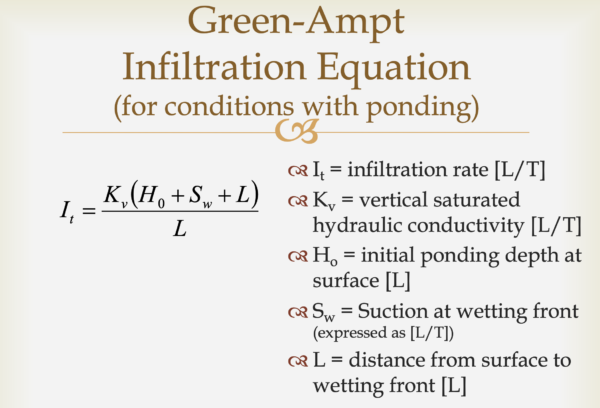
The main Green-Ampt Equation to know (slide 42-44)
Concerned I might be overwhelming students with Green-Ampt derivations, I wanted to draw their attention back to a fairly simple form presented in my course slides. Make sure you’ve followed the slides and videos enough to know where K and L come from and why Sw and Ho are in the equation.
Measuring infiltration capacity in the field (slides 45-48)
The above link takes you to a blog post where I explain how double ring infiltrometers and Guelph permeameters work, and remind you about the definitions of infiltration capacity and equilibrium infiltration capacity. I also have some nifty videos of them in action, including one of my students from a previous year.
Assessments
Students’ understanding of the material in this unit was assessed in three ways:
- a problem set with four parts: (1) presenting soil moisture data time series and asking for interpretation of it; (2) using an Excel spreadsheet (that I provide) with the Green-Ampt equation embedded to change soil properties and assess the effects on infiltration; (3) using the same Excel spreadsheet to conduct a sensitivity analyses on the effects of initial water content and rainfall rate and explain their results; and (4) sending them to the Web Soil Survey and a target area of interest to assess what information relevant to the Green-Ampt equation they can find readily versus what requires assumptions of appropriate values (e.g., from a textbook table) or specialized measurements.
- a 10 question multiple choice quiz that I wrote to align with the learning objectives. There were more than 10 questions in the test bank and students could take the quiz 2 times.
- questions on a midterm exam that spanned evapotranspiration and this unit.
Special thanks to…
Many of the amazing videos for this unit were made by Dr. John Selker of Oregon State University. You can learn even more about soil hydrology and biophysics from him at https://www.youtube.com/channel/UCoMb5YOZuaGtn8pZyQMSLuQ/playlists.
And thanks also to Dr. Todd Walters of Cornell University for his clear images and explanations linked above. You’ll see more from him in the next unit on streamflow generation mechanisms.
Please respect my work
This work (my videos and blog posts) are licensed under an Attribution-NonCommercial-NoDerivs 3.0 Unported (CC BY-NC-ND 3.0). That means that you need to give appropriate credit if you use or modify anything I’ve posted here. It also means that you can’t use the material for commercial purposes. If you want to use other resources I’ve listed above, please respect the rights of the originators. If you want to use my sequencing of topics and resources in your class, by all means, go ahead.


Nice plan for content warnings on Mastodon and the Fediverse. Now you need a Mastodon/Fediverse button on this blog.